The ultimate value of an RNA-Seq experiment comes from data analysis. Next generation sequencing (NGS) experiments generate a tremendous amount of data which—unlike Sanger sequencing results—can’t be directly analyzed in any meaningful way. With help from modern computing, scientists aim to extract as much useful information as possible from RNA-Seq results while avoiding misinterpretation or bias. Selecting the right analytical approach along with an appropriate set of bioinformatics tools is key to this objective. Many powerful software programs are available, often for free, that can slice and dice the data in myriad ways. For newcomers, analyzing huge NGS datasets can be intimidating, and knowing where to start isn’t obvious. Here, we provide a brief introductory tutorial to RNA-Seq bioinformatics as well as resources for more in-depth exploration. We’ll focus our discussion on short-read Illumina® sequencing data, which is commonly used for RNA-Seq experiments.
What You Need for RNA-Seq Analysis
- Hardware
- Linux environment or server
- Accessed via shell terminals, such as PuTTY or MobaXterm
- Can use a virtual machine on Windows
- 32GB RAM recommended if working with larger genomes
- 1TB storage or higher recommended for smaller projects
- Linux environment or server
- Software
- Skills
- Using the command line
- Installing and executing software
- Navigating file trees
- Scripting
- Bash, Python, and/or Perl
- R scripting
- Using the command line
Most bioinformatics tools for NGS analysis have been developed for the Linux environment, so you’ll need to know how to use the Linux command line to install software, execute programs, and navigate file trees. Some familiarity with scripting is also required to parse data, format output files, and execute some analyses. To speed up computation, we recommend using a grid cluster, if available, to analyze multiple samples at the same time.
Analyzing RNA-Seq Data
Let’s walk through a typical bioinformatics workflow to illustrate step by step how RNA-Seq data is processed with the goal of differential gene expression analysis.
- Starting with the Linux command line
- Check quality with FastQC
- Trim reads with Trimmomatic
- Align reads to the reference genome with STAR
- Calculate gene hit counts with FeatureCounts
- Compare hit counts between groups with DESeq2
1. Starting with the Linux command line
First, switch to the FASTQ directory. Use the cd command (i.e., change directory) followed by the path where the FASTQ files are stored.
cd /path/to/folder_name/Next, you can check the FASTQ files by using the ls command (i.e., listing), which shows the contents of the current working directory.
Data files from sequencing providers are typically compressed and have the extension “.fastq.gz”. These files contain structured information about individual NGS reads—a unique identifier, the called bases, and the associated quality scores—which can be viewed using the zmore command. In this format, however, the raw data is not particularly useful to examine directly by eye, given the sheer number of reads—often in the millions.
Lastly, you can make an output directory using the mkdir command (i.e., make directory). Output files can be stored here.
mkdir /path/to/output_folder/For the next steps in the workflow, we’ll provide general commands for the processes described. However, please check the documentation that accompanies each software program to tailor it to your data, computer system, and analytical requirements. We also recommend viewing our recorded workshop “Bioinformatics for RNA-Seq” which provides screenshots of actual analyses along with helpful commentary and insights.
2. Check quality with FastQC
Run FastQC to check the raw data quality.
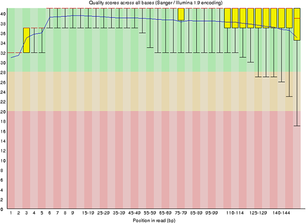
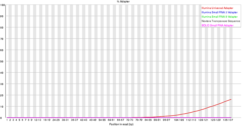
fastqc sample_01.fastq.gz --extract -o /path/to/output_folderThe output contains graphs and statistics about the raw quality, including quality scores, GC content, adapter percentage, and more. Below are two examples of the output files.
3. Trim reads with Trimmomatic
Poor-quality regions and adapter sequences should be trimmed from the reads before further analysis. Since Trimmomatic has an executable JAR file, you’ll need to use Java to execute it rather than doing so directly in the command line.
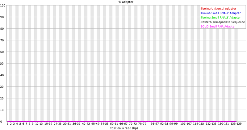
java -jar trimmomatic-0.39.jar PE input_forward.fastq.gz input_reverse.fastq.gz output_forward_paired.fastq.gz output_forward_unpaired.fastq.gz output_reverse_paired.fastq.gz output_reverse_unpaired.fastq.gz ILLUMINACLIP:TruSeq3-PE.fa:2:30:10:2:keepBothReads LEADING:3 TRAILING:3 MINLEN:36Run FastQC again on the trimmed treads to confirm that the new quality is acceptable (see figures below).

4. Align reads to the reference genome with STAR
First, index the reference genome using STAR to prepare it for alignment. Adding gene annotation information to the reference genome will facilitate alignment of RNA-Seq reads across exon-intron boundaries. This indexing step is only required once; you can then use the indexed genome repeatedly in future analysis.
STAR genomeGenerate --genomeDir <genome output directory> --genomeFastaFiles <input genome FASTA file> --sjdbGTFfile <annotation file>Then, align the reads. The default output for the STAR aligner is a SAM file, which should be converted to a BAM file for downstream use.
STAR --genomeDir <directory with indexed genome> --readFilesIn <trimmed fastq file> --outFileNamePrefix <sample name> --outSAMtype BAM UnsortedCheck the mapping statistics in the [sample_name]Log.final.out file to ensure the BAM file was generated properly and the reads align to the genome correctly. Uniquely mapped reads are the most useful for expression analysis, as there is high confidence in which loci they represent. In general, >60-70% for the “uniquely mapped reads %” metric is considered good; a significantly lower value warrants further investigation.
Lastly, use Samtools to sort and index the BAM files. Organizing the reads by position within the BAM file is needed for downstream analysis.
samtools sort sample.bam -o sample.sorted.bam samtools index sample.sorted.bam5. Calculate gene hit counts with FeatureCounts
Use FeatureCounts to calculate the number of reads per gene. We suggest counting only uniquely mapped reads that fall within exons. Reads that align to introns or intergenic regions may represent genomic DNA contamination or pre-mRNA (i.e., unspliced mRNA). We recommend using gene ID as the identifier in the summary table since other identifiers, such as gene symbol, may not be available for all loci.
featureCounts -a annotation_file.gtf -o sample.counts.txt --largestOverlap -t exon -g gene_id sample.sorted.bamNext, check the stats file to validate the quality of the data, in particular the number of assigned reads. About 15 to 20 million reads per sample are typically recommended for RNA-Seq analysis, but it’s possible to use fewer reads. The target number of reads depends on the objectives of the project and the species under investigation.
6. Compare hit counts between groups with DESeq2
First, you’ll need to merge the hit counts from all samples into a summary table using R scripting or Excel™ (see example below).
Summary of Hit Counts
| ID | Control1 | Control2 | Control3 | TreatmentA-1 | TreatmentA-2 | TreatmentA-3 |
|---|---|---|---|---|---|---|
| ENSMUUSG00000104123 | 722 | 376 | 455 | 1158 | 611 | 270 |
| ENSMUUSG00000102948 | 0 | 0 | 1 | 2429 | 2014 | 2514 |
| xxx | xxx | xxx | xxx | xxx | xxx | xxx |
| And so on | … | … | … | … | … | … |
Then, create a table that lists the sample names and their group assignments (see example below). This information will instruct DESeq2 how to compare the samples. Both tables can be outputted as tab-delimited text files.
Group Assignments Table
| SampleID | Condition |
|---|---|
| Control1 | Control |
| Control2 | Control |
| Control3 | Control |
| TreatmentA-1 | TreatmentA |
| TreatmentA-2 | TreatmentA |
| TreatmentA-3 | TreatmentA |
Before working with DESeq2, install the following libraries in R.
install.packages(c(“DESeq2”, “Biobase”, “gplots”, “ggplot2”, “RColorBrewer”, “pheatmap”, “matrixStats”, “lattice”, “gtools”, “dplyr”)In R, import the count data and sample grouping files.
myCountTable <- “raw_counts.txt” myCondition <- “testCondition.txt”Then, execute the DESeq2 analysis, specifying that samples should be compared based on “condition”.
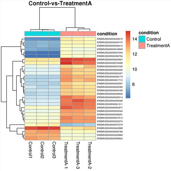
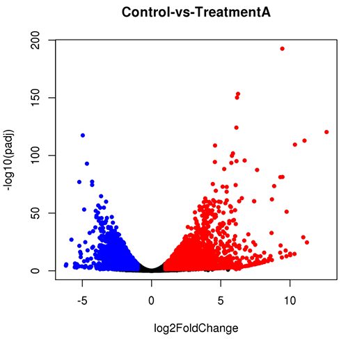
dds = DESeqDataSetFromMatrix(myCountTable, myCondition, design = ~ Condition) dds <- DESeq(dds)Below are examples of several plots that can be generated with DESeq2. A comprehensive tutorial of this software is beyond the scope of this article. We recommend reviewing the DESeq2 manual for an in-depth explanation of how to perform each type of analysis and which parameters can be adjusted.

Key Takeaways
- The barrier to entry for bioinformatics is relatively low: access to a Linux system with enough memory and some familiarity with scripting (the software is available for free online)
- RNA-Seq data analysis is a step-by-step process and it’s best practice to check the quality of the output data before using it as input for the next step
- Analysis can be sped up with automation via scripting and grid computing
Conclusion
A theme emerges from the workflow above: it’s important to perform quality control checks, where possible, before advancing to the next step. Detecting errors or issues early will save substantial time and effort down the line. With a bit of training and practice, virtually any scientist can get started with RNA-Seq data analysis. Once you feel comfortable with each step, you can create scripts to build pipelines for streamlined analysis. Although we focused on the mechanics of performing data analysis here, it’s imperative that you understand the statistical principles behind the analyses to interpret your data properly.
For a deeper dive into RNA-Seq bioinformatics, check out our on-demand educational workshop. It explores the bioinformatics pipeline, explains NGS results, addresses common challenges, and answers frequently asked questions regarding RNA-Seq analysis.

